Regression and
Survival Analysis

Zarathu

Executive Summary

	Default	Repeated Measure	Survey
Continuous	Linear regression	GEE	Survey GLM
Event	GLM (logistic)	GEE	Survey GLM
Time & Event	Cox	Marginal Cox	Survey Cox
0,1,2,3 (rare event)	GLM (Poisson)	GEE	Survey GLM

Dataset

Linear regression

Continuous

Concept

It predicts a continuous outcome (dependent variable) by fitting the best possible straight-line relationship to one or more explanatory variables (independent variables).

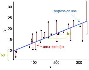
\[Y = \beta_0 + \beta_1 X + \epsilon\] Estimate \(\beta_0\), \(\beta_1\) by minimizing sum of squared errors

\(Y\) must be continuous & normally distributed
\(X\) can be continuous or categorical
- If continuous: same as correlation analysis
- If binary: same as t-test with equal variance

Case 1. X is continious (Age → Node)

This regression estimates how age affects nodes (number of affected lymph nodes).

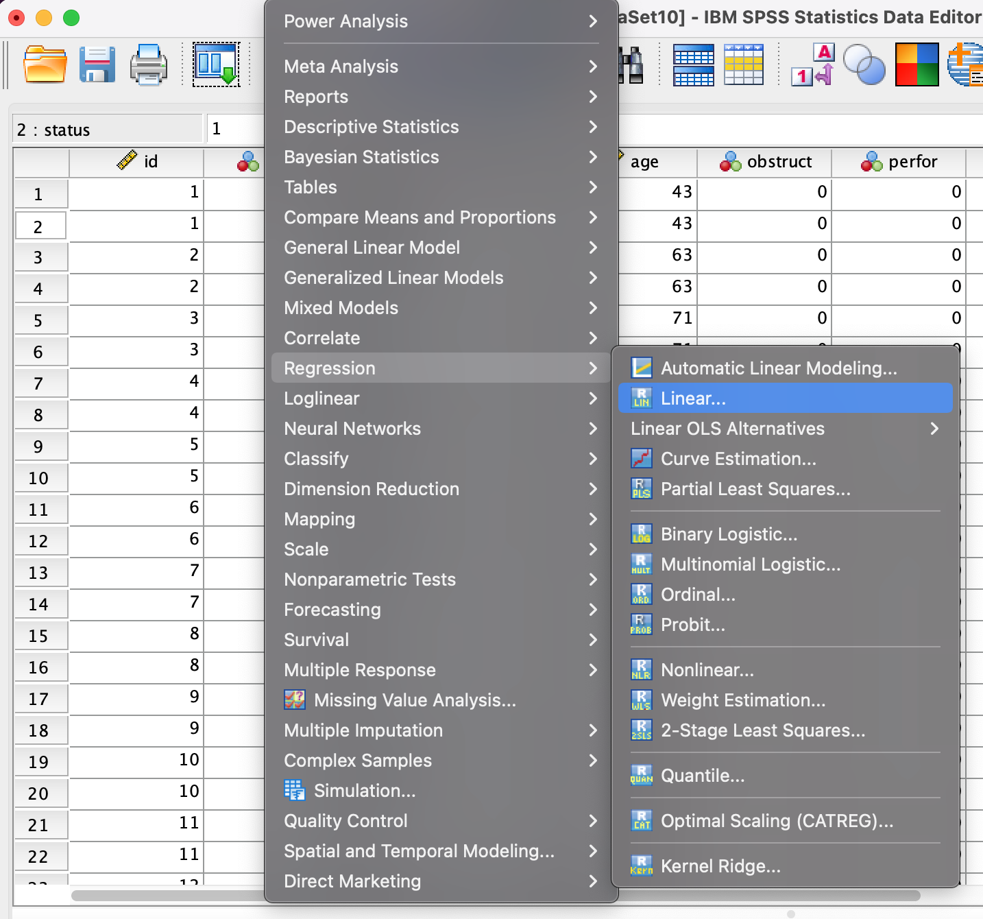
Step 1

Go to Analyze → Regression → Linear…

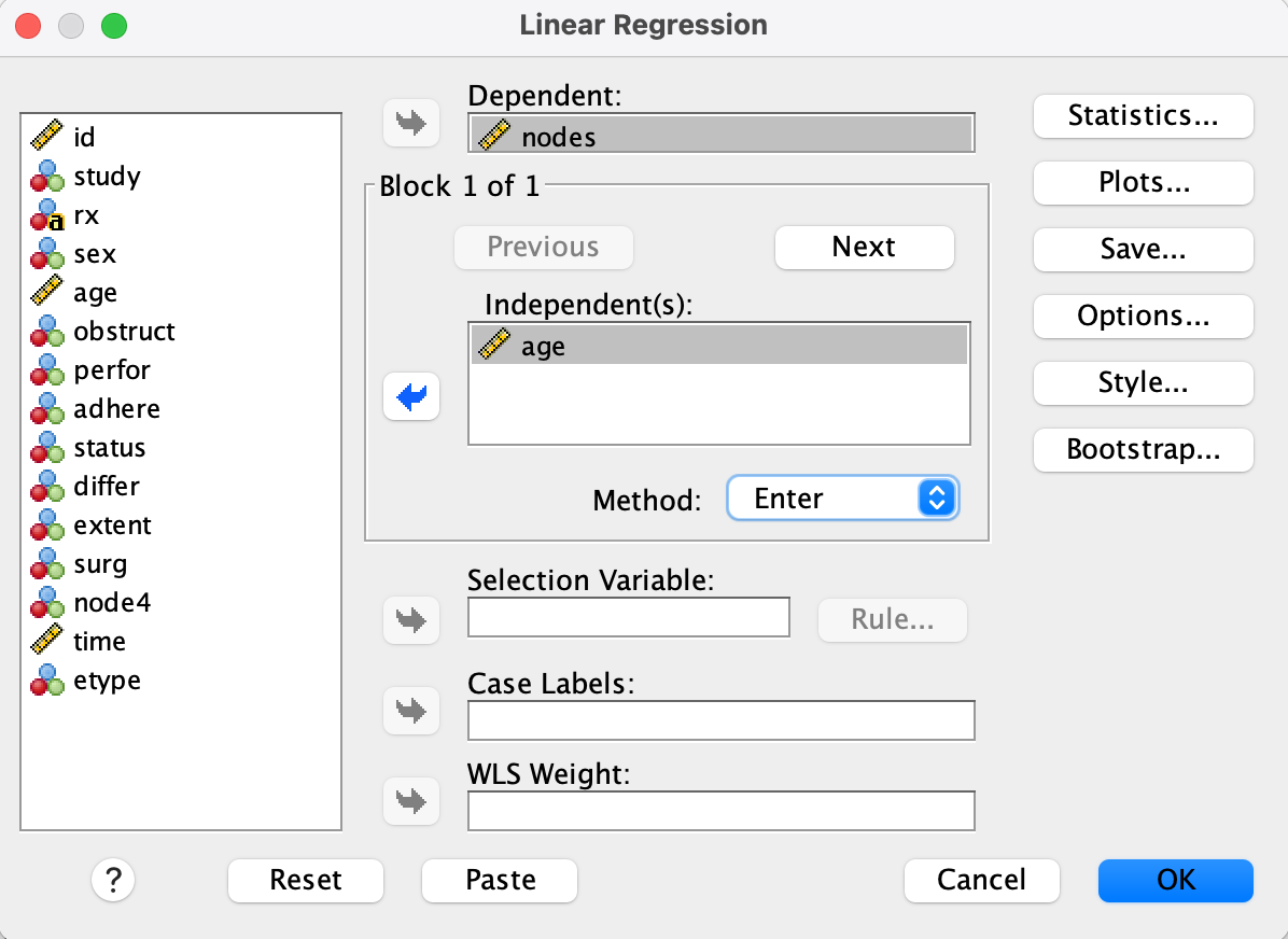
Step 2

Set nodes as the Dependent variable and age as the Independent(s) variable.

Result

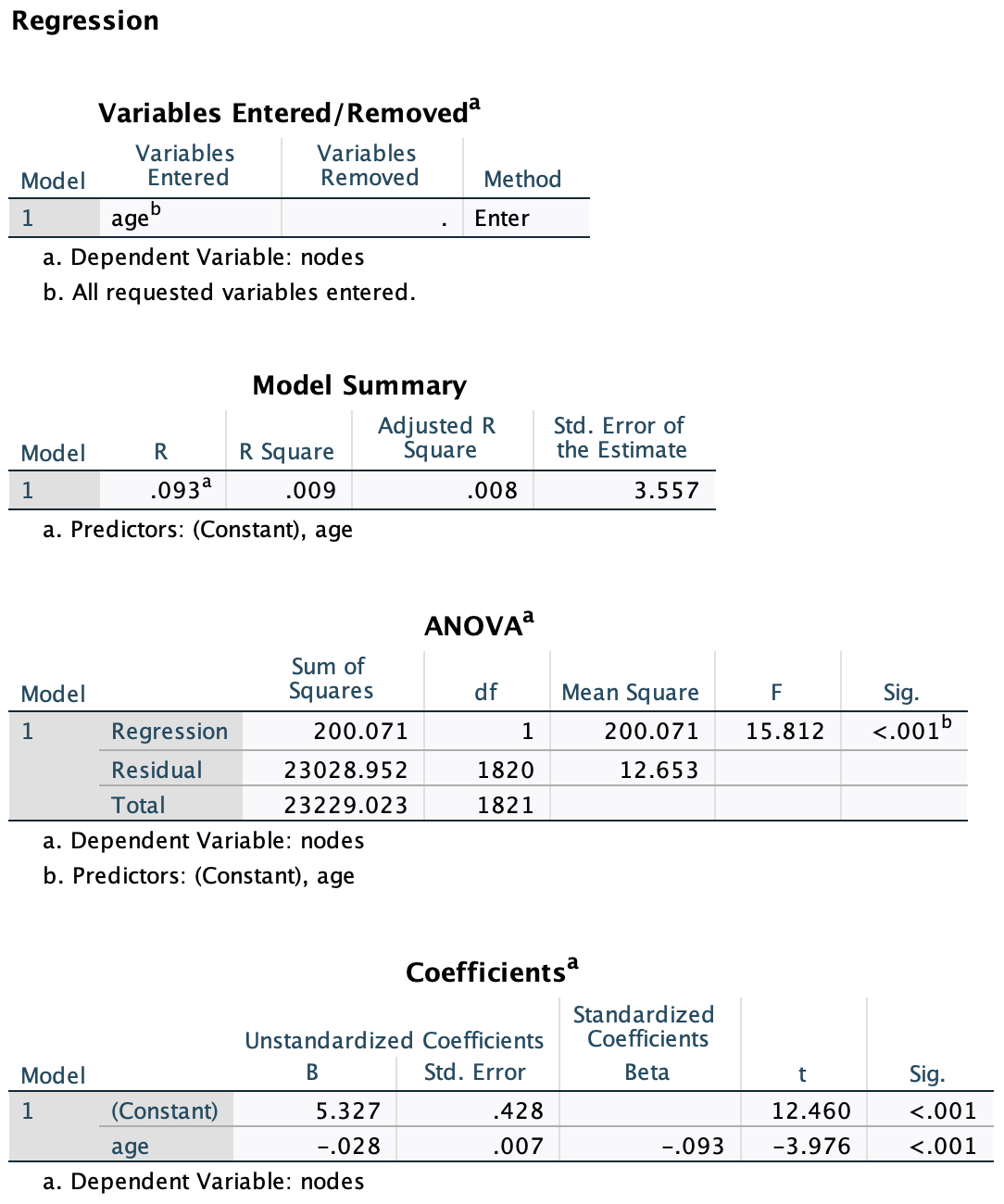
R = .093, R² = .009: Very weak linear relationship
Unstandardized coefficient for age = -0.028, p < .001

As age increases by 1 year, the number of nodes is expected to decrease by 0.028. The relationship is statistically significant but weak.

Case 1. X is continious (Node → Age)

This reverses the regression direction, predicting age from nodes.

Step 1

Go to Analyze → Regression → Linear…
Set age as the Dependent variable and nodes as the Independent(s) variable.

Result

R = .093, R² = .009: Same strength as the previous model (symmetric)
Unstandardized coefficient for nodes = -0.309, p < .001

Although both models are statistically significant (p < .001), the effect size (R² ≈ 0.009) is very small. This indicates that only about 0.9% of the variance in either variable is explained by the other.

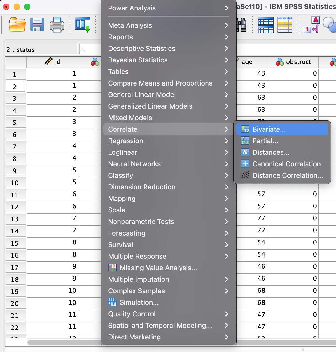
Case 1 = Bivariate Correlation

We can also use the Bivariate Correlation function to test linear association between two continuous variables.

Step 1

Analyze → Correlate → Bivariate…

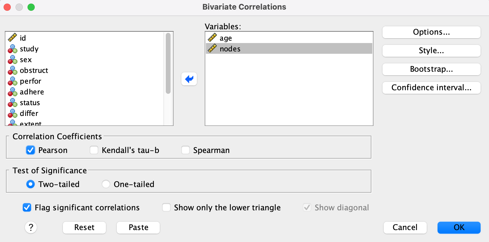
Step 2

Move age and nodes into the Variables box
Select Pearson as the correlation coefficient
Choose Two-tailed test of significance

Result

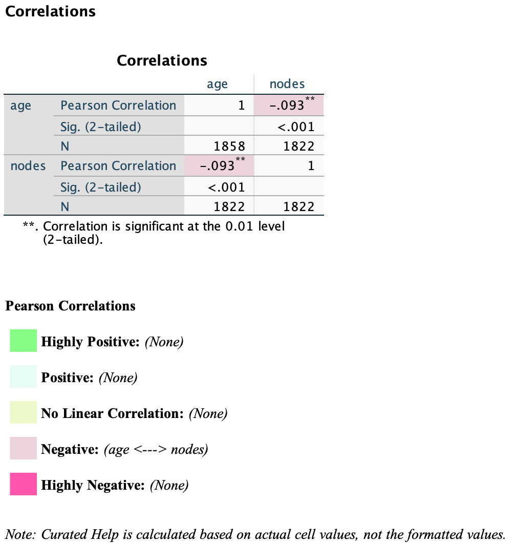
Pearson correlation: r = -0.093
p-value: < .001 → statistically significant
Sample size: N = 1822

There is a weak negative, yet statistically significant, correlation between age and nodes.

Case 2. X is binary (Sex → Time)

This analysis fits a linear regression model where time is predicted by sex.

Step 1

Go to Analyze → Regression → Linear…

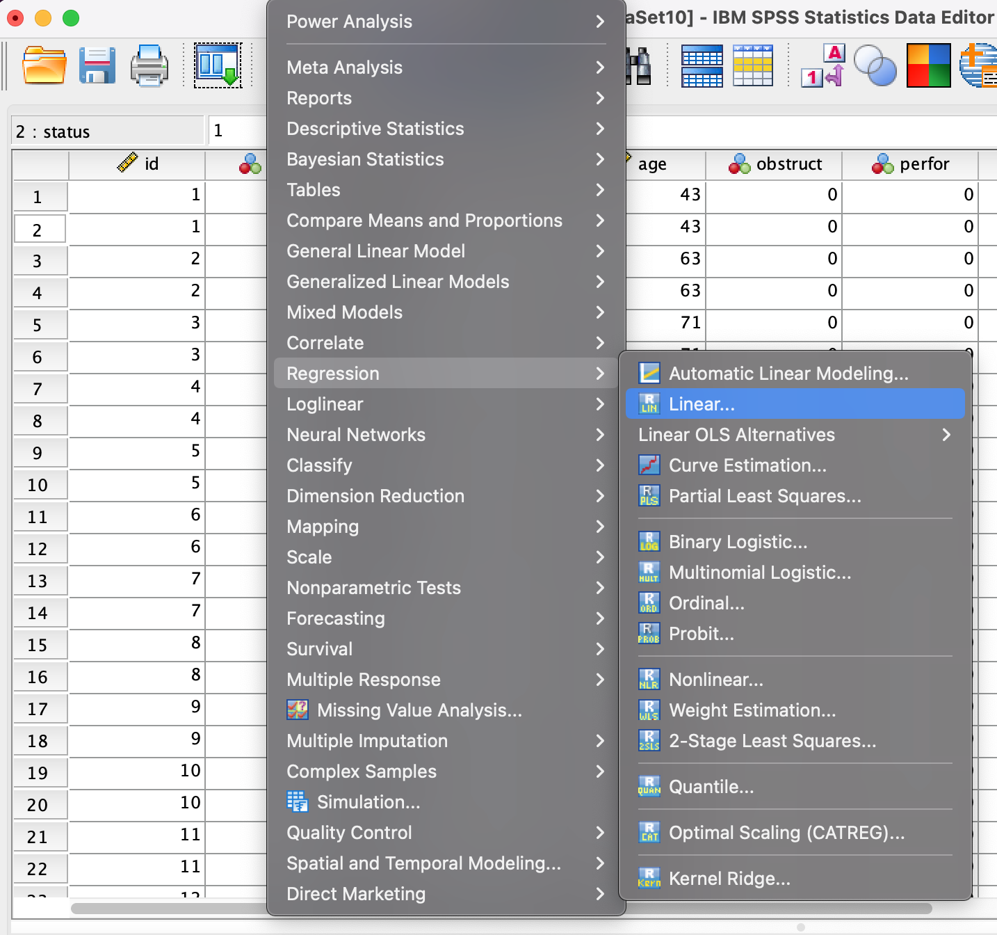
Step 2

Set time as the Dependent variable and sex as the Independent(s) variable.

Result

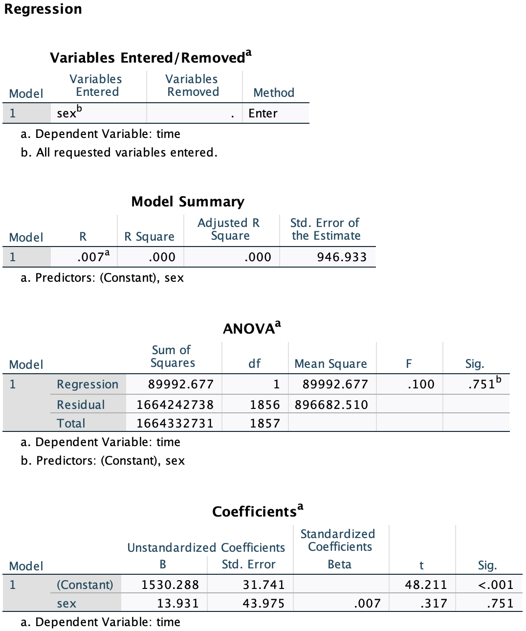
There is no statistically significant association between sex and time.

Case 2 = Independent Samples T-test

T-test and Simple Linear Regression are equivalent when comparing 2 groups.

To compare the variable time between male and female groups, use a t-test in SPSS:

Result

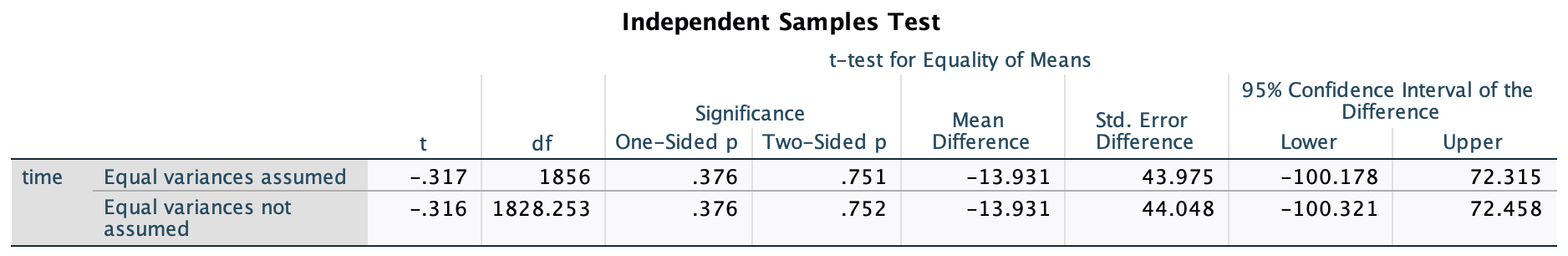
t = -0.317, df = 1856, p = 0.751
No statistically significant difference in mean time between groups

The regression result is consistent with the t-test. Therefore, t-test provides the same result as regression when the predictor has only two levels, and is more intuitive.

Case 3. X is categorical with 3↑ values (rx → Time)

Change string to numeric

The variable rx includes three treatment groups:

1 = Lev
2 = Lev+5FU
3 = Obs (reference)

In SPSS, linear regression does not automatically treat string variables as categorical. To include a categorical variable like rx in a regression model, we must first convert it to numeric.

Step 1

Use Automatic Recode → Numeric values starting from 1

1 = Lev, 2 = Lev+5FU, 3 = Obs

Now that rx_new is numeric, SPSS will automatically create dummy variables when used in regression, BUT it will use the lowest number as the reference group (e.g., 1 = Lev).

To change the reference group…

Step 2

Create two dummy variables:

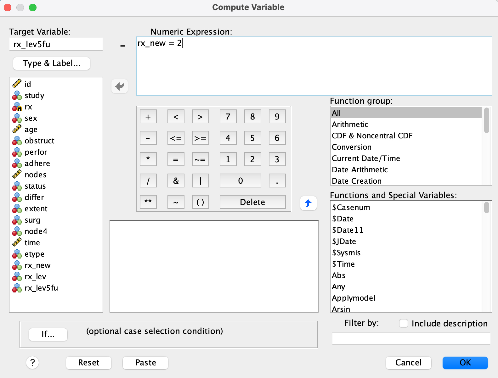
Go to Transform → Compute Variable…
rx_lev = 1 if rx_new == 1, else 0

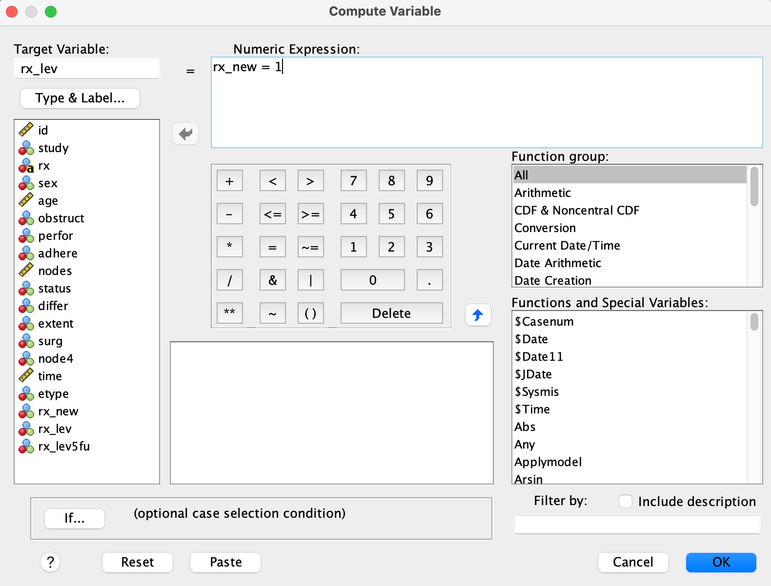
rx_lev5fu = 1 if rx_new == 2, else 0

The reference group (row where all dummy variables are 0) is Obs, which is not coded explicitly.

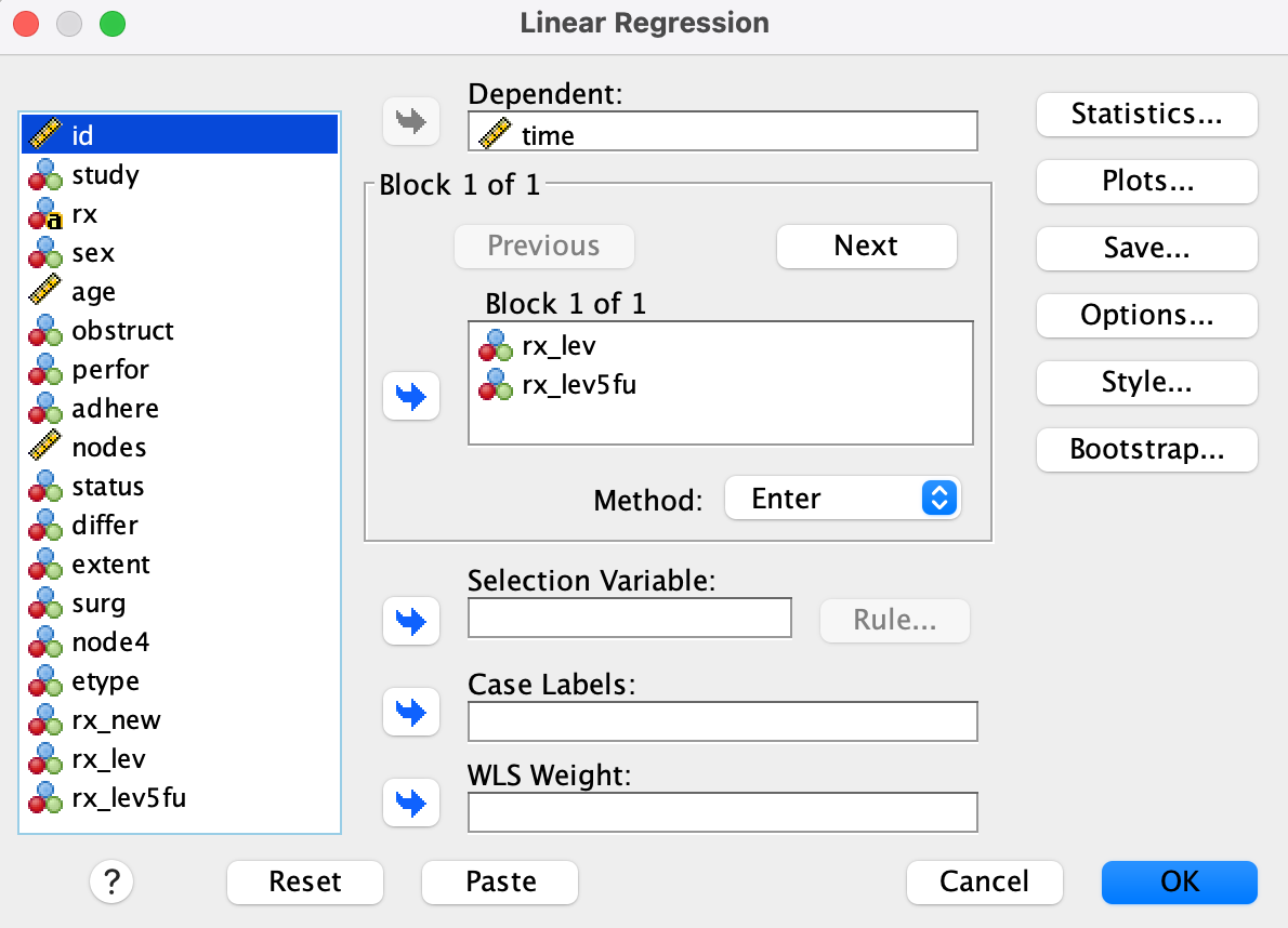
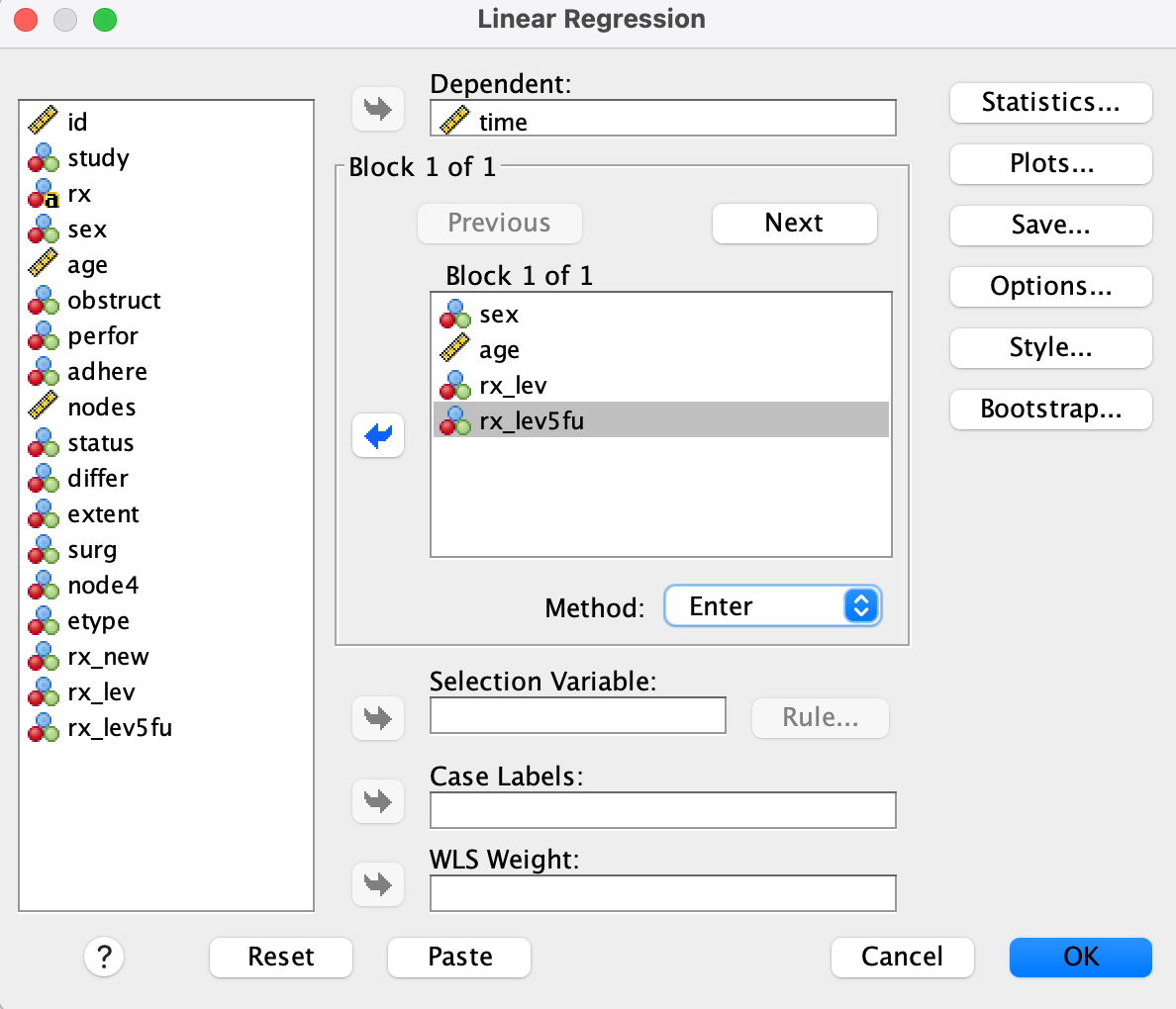
Step 3

Use Analyze → Regression → Linear

Dependent variable: time
Independent variables: rx_lev, rx_lev5fu

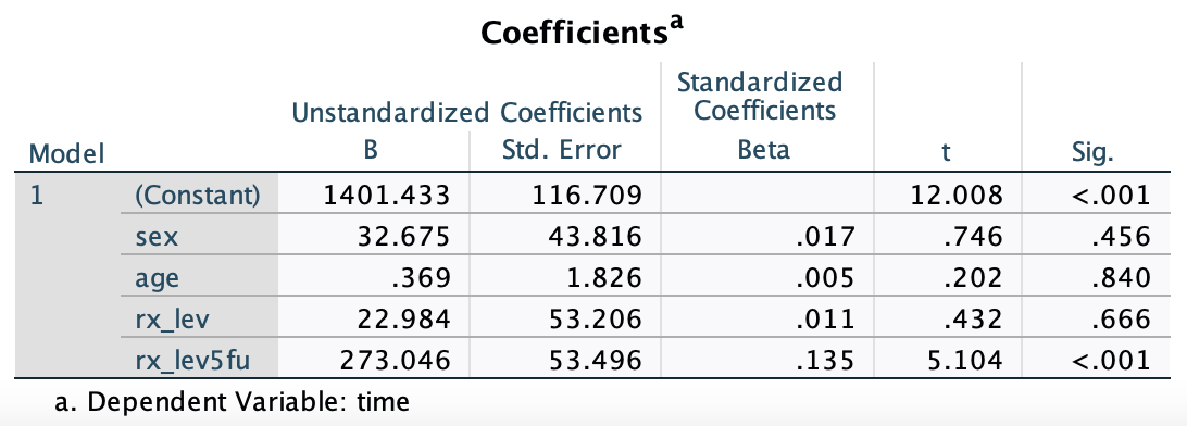
Result

The constant is the mean for the Obs group.
Coefficients show the difference from Obs:

rx_lev = difference between Lev and Obs
rx_lev5fu = difference between Lev+5FU and Obs

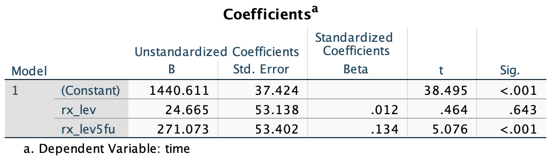
Only rx_lev5fu shows a significant difference (p < .001)

Case 3 is same to One-Way ANOVA

We can also use ANOVA to test whether any of the rx_new groups differ overall.

Step 1

Use Analyze → Compare Means → One-Way ANOVA

-   Dependent = `time`
-   Factor = `rx_new`

Step 2

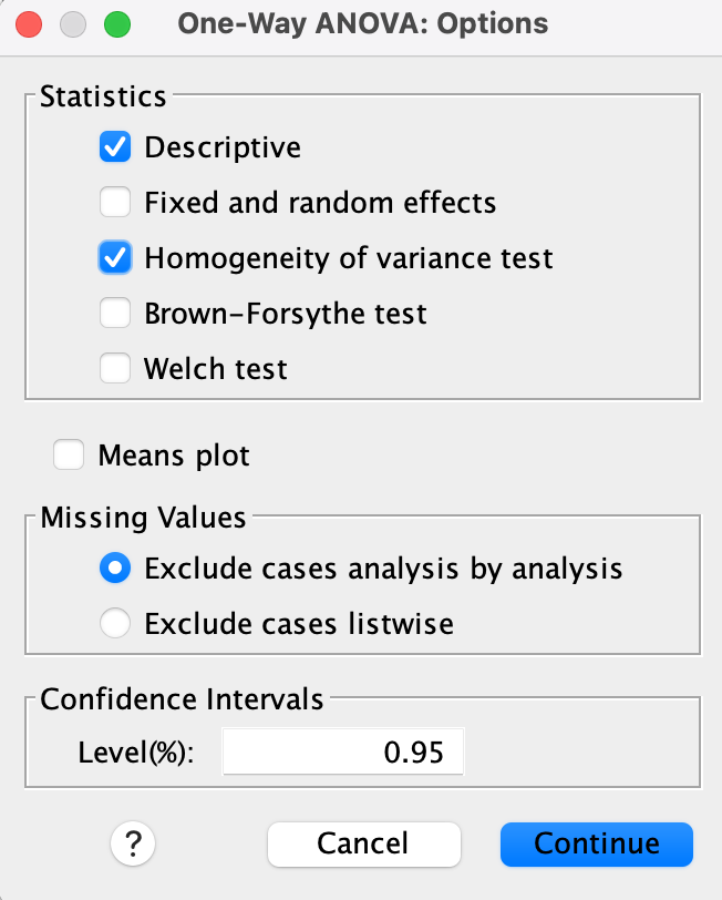
Options → Check Homogeneity of variance test (Levene’s test)

Result

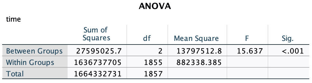
This gives an overall p-value for overall group comparison.

Case 4. multiple X

\[Y = \beta_0 + \beta_1 X_{1} + \beta_2 X_{2} + \cdots + \epsilon\]

Interpretation of \(\beta_1\): When adjusting for \(X_2\), \(X_3\), etc., a one-unit increase in \(X_1\) leads to an increase of \(\beta_1\) in \(Y\).

In academic papers, it is common to present results both before and after adjustment. This allows comparison of crude vs. adjusted effects.

Unadjusted

Analyze each variable one at a time:

Go to Analyze → Regression → Linear
Set time as Dependent
Add one predictor (e.g., sex) to Independent(s)

Adjusted

Control for multiple variables:

Set time as Dependent
Add all predictors (e.g., sex, age, rx) to Independent(s)

Result

Logistic regression

Event

Concept

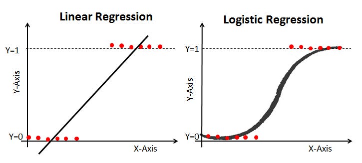
It is used to predict a categorical outcome by estimating its probability. Unlike linear regression, this model uses a logistic (=sigmoid) curve to ensure the output is always constrained between 0 and 1. Internally, it predicts the log-odds of the event, ln(P/(1−P)), and this can be then mathematically converted back into the final probability (P).

\[\begin{aligned} \ln(\frac{p}{1-p}) &= \beta_0 + \beta_1 X_1 + \beta_2 X_2 + \cdots \\\\\\ P(Y = 1) = \frac{\exp{(X)}}{1 + \exp{(X)}} &= \frac{\exp{(\beta_0 + \beta_1 X_1 + \beta_2 X_2 + \cdots)}}{1 + \exp{(\beta_0 + \beta_1 X_1 + \beta_2 X_2 + \cdots)}} \\\\ \end{aligned}\]

Interpretation of \(\beta_1\): When adjusting for \(X_2\), \(X_3\), etc., a one-unit increase in \(X_1\) results in an increase of \(\beta_1\) in \(\ln\left(\frac{p}{1 - p}\right)\), therefore \(\frac{p}{1-p}\) increases by a factor of \(\exp(\beta_1)\).

An Odds Ratio (OR) is a measure of association that compares the odds of an event occurring in one group to the odds of a different group. So, in other words, the Odds Ratio = \(\exp(\beta_1)\)

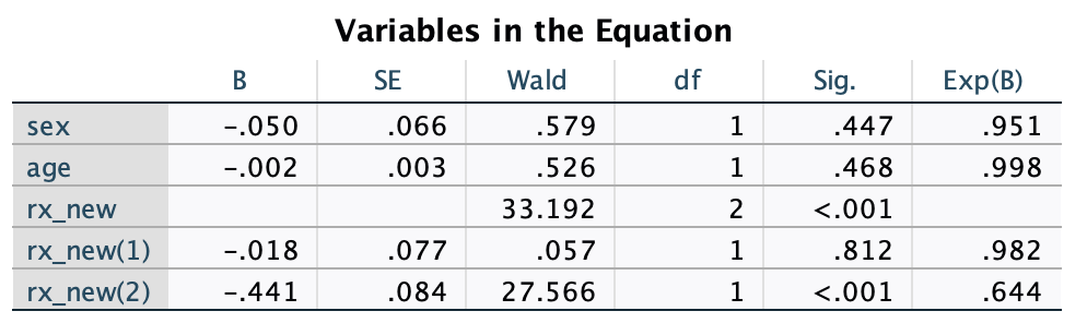
Case 5. Sex, Age, rx_new → status

Step 1

Go to Analyze → Regression → Binary Logistic...
Move status to the Dependent box, sex, age, and rx_new into the Covariates box.

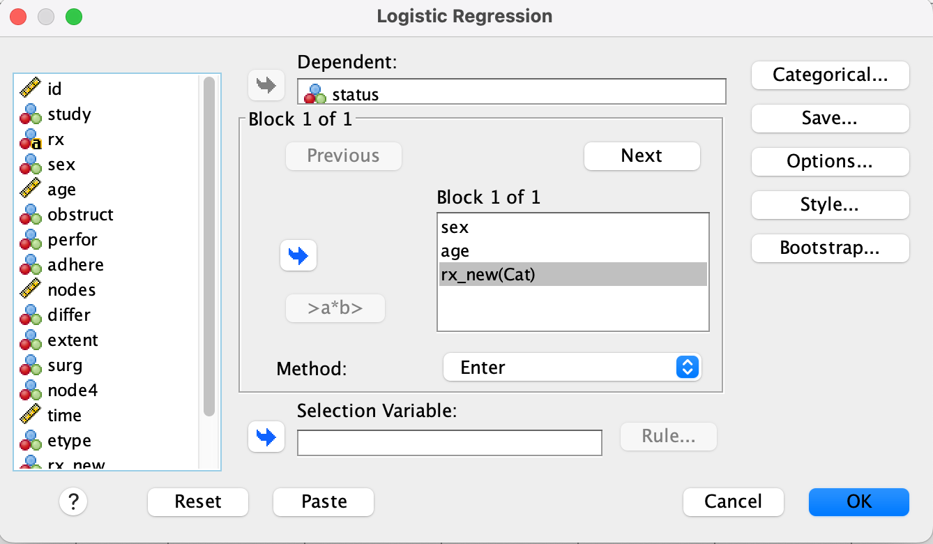
Step 2

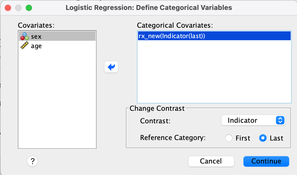
Click Categorical…
Select rx_new, move to Categorical Covariates
Set Reference Category to Last (e.g., Obs)

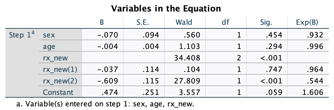
Result

Exp(B) gives odds ratios.

Survival analysis

Time & Event

Concept

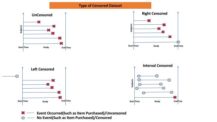
Survival analysis focus on the duration until a specific event of interest such as death occurs. A characteristic of this analysis is censoring, which occurs when the event has not been observed for some subjects by the end of the study, or when subjects are lost to follow-up. Most data are right-censored: the individual either died on day or survived up to day.

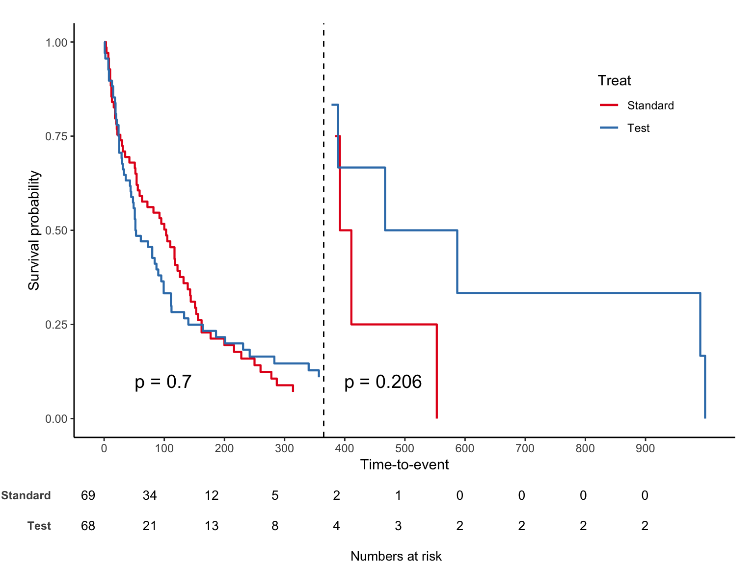
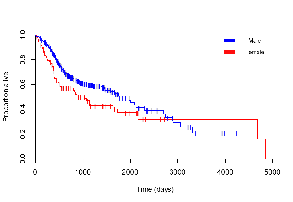
1. Kaplan-meier plot

The first step in any survival analysis is “How is this group surviving over time?” The Kaplan-Meier estimator is the most common method used to answer this.

It provides an estimation of the Survival Function, S(t), which is the probability that an individual will survive past time t. So the resulting Kaplan-Meier curve is a step function. The survival probability remains flat until an event occurs, at which point the curve drops.

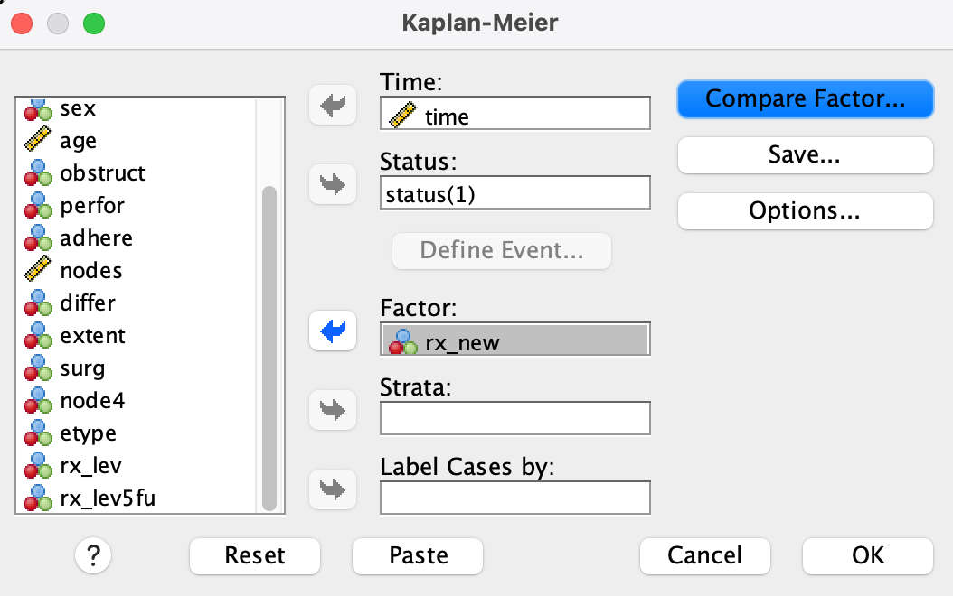
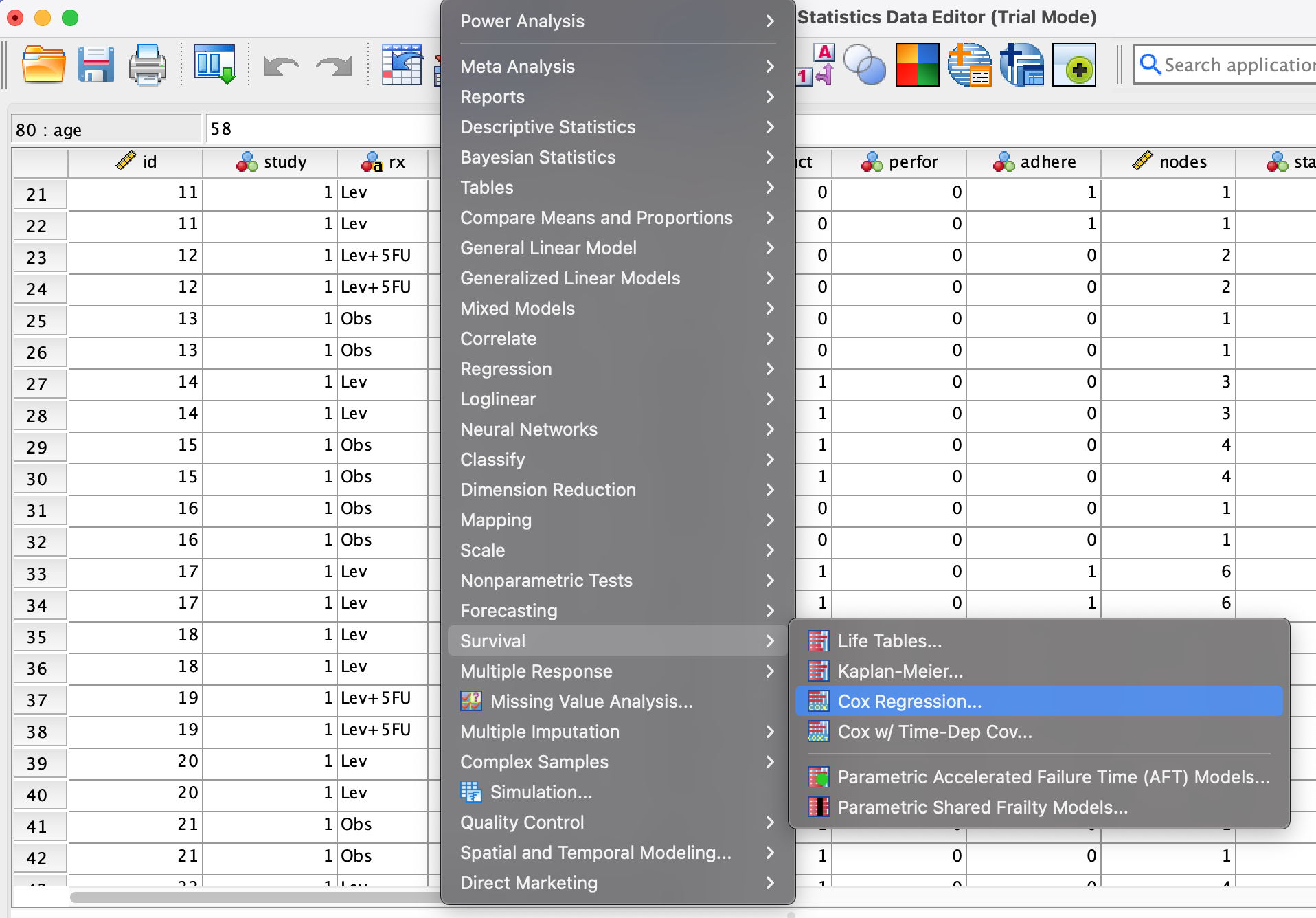
Step 1.

Go to Analyze → Survival → Kaplan-Meier…
Set time as Time, status(1) as Status, rx_new as Factor

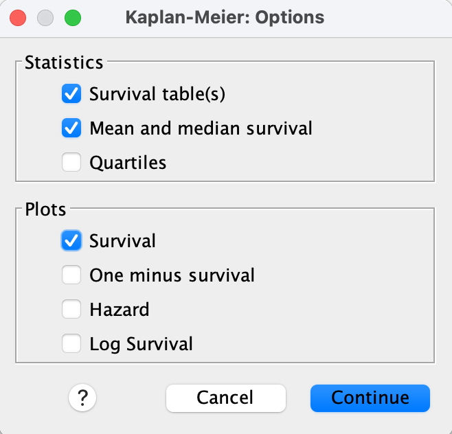
Step 2.

Click Options → Check: Survival table(s) , Mean and median survival , Survival plot

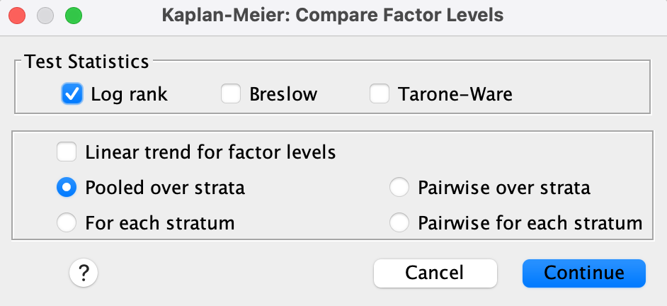
Step 3.

Click Compare Factor… → Check: Log rank, Pooled over strata

Step 4.

Click OK to see: Kaplan–Meier plot with censored cases (+), Log-rank p-value comparing survival curves

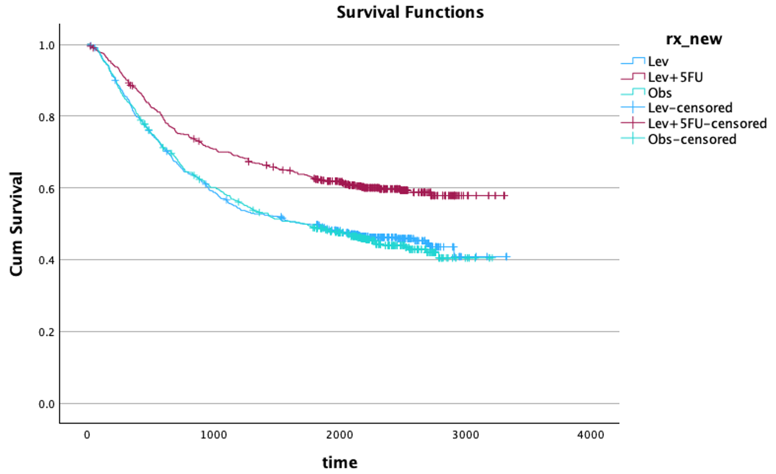
It is usually accompanied by the log-rank test p-value to compare survival between groups.

Calculation

\[ \begin{aligned} P(t) &= \frac{\text{Survived at } t}{\text{At risk at } t} \quad \text{(Interval survival)} \\\\ S(t) &= S(t-1) \times P(t) \end{aligned} \]

A Kaplan–Meier curve is built by chaining together little “survival chances” at each time when at least one death happens. Start with everyone alive at time zero and imagine the survival probability is 1. At each event time, look only at the people who were still under observation just before that moment—the “risk set.” The step size is simply the fraction of that group who make it past the event time. We multiply these fractions across event times to keep updating the curve. Censored observations don’t cause a drop; they only shrink the risk set for the future.

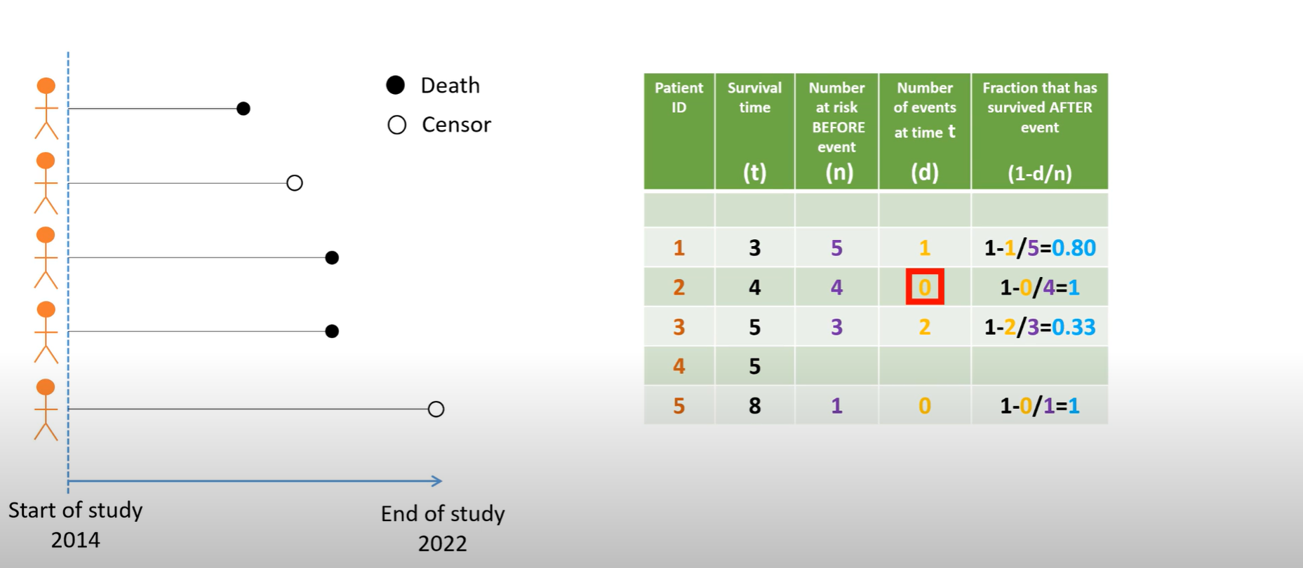
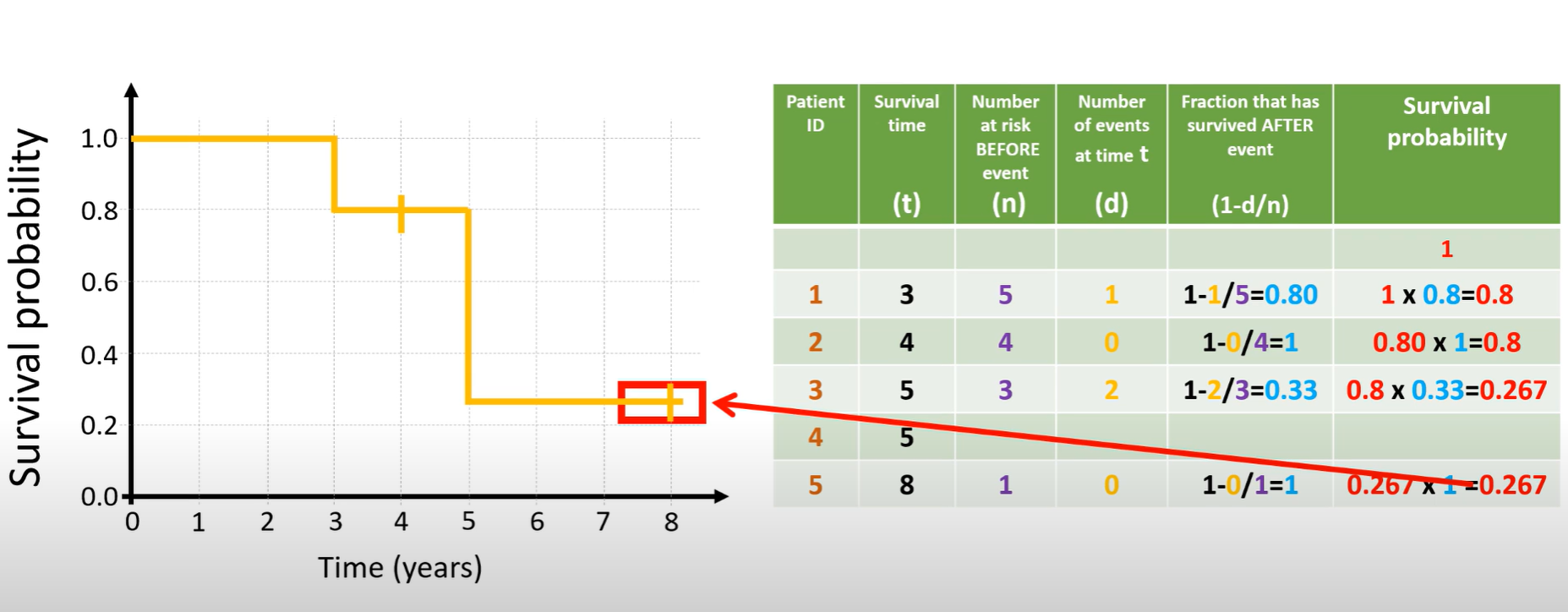
Now apply that idea to the figure. Five people begin. At time 3, one person dies while five were still at risk, so four out of five get past time 3; the curve steps down to 0.80. At time 4, someone is censored. Because no one dies, the curve stays flat at 0.80, but the risk set for later times is now smaller. By time 5, three people are still under observation and two die there; only one of those three gets past time 5, so we scale the curve by one-third, landing around 0.27. At time 8, the last person is censored, so nothing changes numerically—the curve remains about 0.27 through study end.

Read this way, the KM plot is a staircase that only steps down on death times. Each step reflects “what fraction of those still being followed just before this time survived beyond it,” and the final height (about 0.27 here) is the estimated probability of surviving past the last event time.

2. Cox Proportional Hazards (PH) Model

While KM curves and Log-Rank tests are excellent for comparing groups based on a single categorical variable (like “Treatment A” vs. “Treatment B”), they cannot handle the influence of multiple factors simultaneously (like age, tumor size, blood pressure, and treatment type).

Hazard function: \(h(t)\)

Probability of surviving up to time \(t\) and dying immediately after

The Survival function S(t) described the probability of not having an event by time t. In contrast, the Hazard Function describes the instantaneous risk of the event occurring precisely at time t, given that the individual has survived up to that moment. A high hazard means a high immediate risk of failure.

Cox model

\[ \begin{aligned} h(t) &= \exp({\beta_0 + \beta_1 X_1 + \beta_2 X_2 + \cdots}) \\\\ &= h_0(t) \exp({\beta_1 X_1 + \beta_2 X_2 + \cdots}) \end{aligned} \]

Cox model finally evaluates the Hazard Ratio (HR). When \(X_1\) increases by 1, \(h(t)\) increases by a factor of \(\exp(\beta_1)\). In other words, \[\text{HR} = \exp{(\beta_1)}\]

HR = 1: The covariate has no effect on the hazard.
HR > 1: The covariate increases the risk (e.g., smoking). An HR of 2.0 means that the group has double the instantaneous risk of the event compared to the reference group.
HR < 1: The covariate is protective and decreases the risk (e.g., an effective treatment).

Case 6. Sex, Age, rx_new → time and status

Step 1.

Go to Analyze → Survival → Cox Regression

Step 2.

Set Time = time, Status = status
Click Define Event, enter value = 1

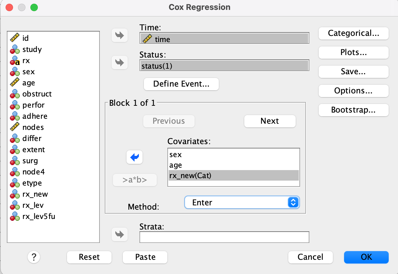
Step 3.

Move sex, age, rx_new to Covariates
Click Categorical, add rx_new, set Reference Category to Last, click Change

Result

Exp(B) = hazard ratio

Proportional Hazards Assumption

The most crucial assumption of this model is the Proportional Hazards Assumption. This means that the HR comparing any two groups must be constant over the entire follow-up time. Visually, this means their survival curves should not cross, and the relative distance between their hazard functions must remain the same over time. No formal test for the assumption is strictly required — it can be checked visually.

Like Kaplan-Meier, statistics are calculated by intervals.
- Assumes similar patterns across intervals (proportional hazards assumption)
Time-independent HR: time is captured only by \(h_0(t)\).
- Model is simple because HR remains constant over time
\(h_0(t)\) is not estimated, which simplifies computation
- But it’s a limitation when building prediction models — you need to estimate \(h_0(t)\) separately

2-1. [Advanced] When Assumption Fail → Landmark-analysis

Landmark analysis is an alternative approach often used to handle specific biases (like “immortal time bias,” where patients must survive long enough to receive a treatment, making the treatment look artificially successful).

This method involves setting a specific time point (=landmark point) and includes only those subjects who survived up to the landmark time. These subjects are then divided into groups based on their status at the landmark (e.g., those who received a transplant by 6 months vs. those who did not). The survival analysis (using KM and Log-Rank) then begins from the landmark point onward, comparing the subsequent survival of these fixed groups.

Analyze separately by dividing time into intervals.

2-2. [Advanced] When Assumption Fail → Time-dependent Cox

If the effect of a variable (its HR) changes over time, we use this model to interact the variable with time, allowing the model to estimate an HR that is a function of time (HR(t)) rather than a single constant.

Piecewise time-dependent Cox model It partitions the observation data into three distinct time interval and estimates a separate and different coefficient (effect) for specific variable within each of those three time intervals.

Call:
coxph(formula = Surv(tstart, time, status) ~ trt + prior + karno:strata(tgroup), 
    data = vet2)

  n= 225, number of events= 128 

                                  coef exp(coef)  se(coef)      z Pr(>|z|)    
trt                          -0.011025  0.989035  0.189062 -0.058    0.953    
prior                        -0.006107  0.993912  0.020355 -0.300    0.764    
karno:strata(tgroup)tgroup=1 -0.048755  0.952414  0.006222 -7.836 4.64e-15 ***
karno:strata(tgroup)tgroup=2  0.008050  1.008083  0.012823  0.628    0.530    
karno:strata(tgroup)tgroup=3 -0.008349  0.991686  0.014620 -0.571    0.568    
---
Signif. codes:  0 '***' 0.001 '**' 0.01 '*' 0.05 '.' 0.1 ' ' 1

                             exp(coef) exp(-coef) lower .95 upper .95
trt                             0.9890      1.011    0.6828    1.4327
prior                           0.9939      1.006    0.9550    1.0344
karno:strata(tgroup)tgroup=1    0.9524      1.050    0.9409    0.9641
karno:strata(tgroup)tgroup=2    1.0081      0.992    0.9831    1.0337
karno:strata(tgroup)tgroup=3    0.9917      1.008    0.9637    1.0205

Concordance= 0.725  (se = 0.024 )
Likelihood ratio test= 63.04  on 5 df,   p=3e-12
Wald test            = 63.7  on 5 df,   p=2e-12
Score (logrank) test = 71.33  on 5 df,   p=5e-14

Executive Summary

	Default	Repeated measure	Survey
Continuous	linear regression	GEE	Survey GLM
Event	GLM (logistic)	GEE	Survey GLM
Time & Event	Cox	marginal Cox	Survey Cox
0,1,2,3 (rare event)	GLM (poisson)	GEE	Survey GLM

Solution without SPSS

https://openstat.ai/

Regression and Survival Analysis

Executive Summary

Dataset

Linear regression

Concept

Case 1. X is continious (Age → Node)

Step 1

Step 2

Result

Case 1. X is continious (Node → Age)

Step 1

Result

Case 1 = Bivariate Correlation

Step 1

Step 2

Result

Case 2. X is binary (Sex → Time)

Step 1

Step 2

Result

Case 2 = Independent Samples T-test

Result

Case 3. X is categorical with 3↑ values (rx → Time)

Change string to numeric

Step 1

Step 2

Step 3

Result

Case 3 is same to One-Way ANOVA

Step 1

Step 2

Result

Case 4. multiple X

Unadjusted

Adjusted

Result

Logistic regression

Concept

Case 5. Sex, Age, rx_new → status

Step 1

Step 2

Result

Survival analysis

Concept

1. Kaplan-meier plot

Step 1.

Step 2.

Step 3.

Step 4.

Calculation

2. Cox Proportional Hazards (PH) Model

Hazard function: \(h(t)\)

Cox model

Case 6. Sex, Age, rx_new → time and status

Step 1.

Step 2.

Step 3.

Result

Proportional Hazards Assumption

2-1. [Advanced] When Assumption Fail → Landmark-analysis

2-2. [Advanced] When Assumption Fail → Time-dependent Cox

Executive Summary

Solution without SPSS

END

Regression and
Survival Analysis